Starting from the ideas behind Meta’s MAIProf, I redesigned capture ownership, process discovery, and trace delivery for Kubernetes.

A training job has already been running for hours when throughput suddenly starts to fluctuate. At that point, the thing you usually want is not to stop the job, add a pile of profiler flags, and try to reproduce the issue. You want to take a snapshot of what is happening right now:

Start capturing for a few seconds, now, and bring back GPU traces from every rank.

On a single machine, this sounds like one profiler call. On Kubernetes, it quickly turns into a distributed systems problem: training processes are spread across nodes, a single Pod may contain multiple torchrun workers, sending a request does not mean Kineto actually accepted it, and a file appearing on disk does not mean it is complete—or that downstream analysis knows which rank it belongs to.

I did not start from scratch. The real starting point was Meta’s 2022 PyTorch Blog post: Performance Debugging of Production PyTorch Models at Meta.

Meta gave me the problem decomposition, not an implementation I could copy

That post describes the overall MAIProf idea: a user submits a profiling request; a Profiling Service discovers the GPU hosts running the training job and broadcasts the request to Monitoring Daemons on those hosts; Kineto generates one trace per GPU, uploads the traces to object storage, and the system analyzes them together afterward.

What mattered most to me was the problem decomposition rather than any individual component: profiling can be an independent service, and a capture should be treated as a job-wide operation rather than something attached to one process.

The public building blocks cover both ends of the pipeline. PyTorch torch.profiler and Kineto handle capture, dynolog provides the daemon-side path, and HTA analyzes traces. What is not public is the orchestration layer in the middle: how to discover a job, expand it into all profiling targets, track request lifecycle, and deliver a set of traces as one trustworthy capture.

More importantly, the public path carries a clear Slurm shape. Kineto uses SLURM_JOB_ID to identify the job, and upstream unitrace.py expands allocation hosts through squeue and scontrol. Kubernetes gives us something different: Pods that are rebuilt, multiple processes inside one container, selectors that can change over time, and a completely different controller failure model. The workload identity, process topology, and failure semantics are different, so the control plane cannot be translated one-for-one.

The per-job coordinator, ephemeral capture state, frozen target snapshots, at-least-once dispatch, and manifest-based delivery described below are therefore Kubernetes-specific trade-offs I made while following the same problem decomposition. They are not claims about Meta’s internal implementation. The profiling-operator described here is not currently open source either; this post is about the reasoning process, not a code release.

There is one more boundary that is easy to blur. MAIProf’s “No source-code change required” does not mean “attach to any arbitrary process after the fact.” My implementation also does not require changes to model source code, but the training workload must be armed at creation time with a hook, environment variables, and a shared directory so that Kineto enters daemon mode. You arm the workload once, then repeatedly trigger captures later without interrupting training.

In the first version, one capture was one CR

The first version followed the most natural Kubernetes Controller design. One capture was a ProfileRun. A central Operator watched it, discovered all target Pods, fanned out to the relevant nodes, and wrote per-rank progress back to status.

The benefits were real. Users could watch progress with familiar kubectl get -w. If the Operator lost leadership, a new leader could recover from state already stored in the API Server. Kubernetes had already solved persistence, watch delivery, concurrent updates, and access control for me. At first, there seemed to be no reason to build something else.

The problem appeared while I was reading through the Reconcile path. The controller had a single worker by default, and fan-out was synchronous. If one node silently dropped packets, one Reconcile could occupy the only worker for a long time. The next item in the queue might not be another rank from the same job. It could be a completely unrelated training job elsewhere in the cluster. A node-local data-plane failure could therefore become a cross-job control-plane stall.

This was not an incident that forced the redesign. It was a risk visible directly from the code path, and I did not want to wait for it to block unrelated workloads in production.

The cheapest fix was obvious: increase MaxConcurrentReconciles, add timeouts to fan-out, and move node calls into goroutines. That would reduce head-of-line blocking, but it would not change the actual boundary of the problem. As long as I wanted a capture to continue across leader failover, I still had to persist the target snapshot, timing origin, deadlines, and per-target state. Every rank transition would still become an API Server write. None of the temporal protocol disappeared.

More workers would only allow more captures to occupy central control-plane resources at the same time. They would not isolate a failure to one job.

That is why I did not stop at “optimize Reconcile.” One capture naturally belongs to one attempt of one training job. Target membership, permissions, archive prefixes, and lifecycle are all job-scoped. The real mistake was not a concurrency setting. It was where orchestration lived.

Then I gave capture back to the job

In the second version, the central Operator only owns the slow path. It discovers training jobs that have profiling capability and creates one coordinator for each (job, attempt). Capture requests go directly to that coordinator. The coordinator expands targets in memory, fans out to node agents, waits for traces, and decides when the capture converges.

The node agent still owns only the things that are inherently local: PIDs, UNIX sockets, dynolog, and files.

                         create / garbage collect
Lifecycle Operator  ------------------------------>  Per-job Coordinator
                                                        ^          |
                                                        |          | fan-out / query
                                             Start /    |          v
                                             Watch      |      Node Agents
                                                        |          |
CLI / Gateway  -----------------------------------------+          v
                                                               stock dynolog
                                                                    |
                                                                    v
                                                              Kineto workers
                                                                    |
                                                                    v
                                                            Node-local traces
                                                                    |
                                                        verify / archive
                                                                    |
                                                                    v
                                                             Shared storage
                                                                    |
Per-job Coordinator  -------- manifests ----------------------------+--> HTA analysis

The benefit of this split was clear. The capture hot path no longer writes to the API Server. One stuck node affects one job instead of the entire cluster. Restarting or re-electing the central Operator does not interrupt captures already driven by a coordinator.

The bill was equally clear, and it was not cheap.

The first version’s native kubectl get -w became a read API on the coordinator. The failover recovery I got for free from CR persistence was not carried over either. If the central Operator changes leaders, nothing happens to an in-flight capture. But if the coordinator itself dies, an unfinished capture is abandoned. A replacement coordinator can only answer Unknown for that old capture.

Every armed job also keeps a coordinator Pod alive, which consumes resources and tenant quota. If a request arrives before the Pod is Ready or before its endpoint exists, there is a cold-start window. The external interface becomes two layers rather than one: a CaptureCoordinator CRD for lifecycle and a gRPC API for individual captures.

The redesign also changed how I think about the Kubernetes API boundary. The API Server is a good place for desired state and slow lifecycle state, but that does not mean every short-lived distributed protocol should be encoded into CR status. The issue is not simply that “the API Server is slow.” The capture hot path, its state ownership, and its failure domain all belong to the job. Persisting them into a global control plane buys cross-failure recovery and cross-job coupling at the same time.

The second version did not remove state from the system. It changed who owns that state and where it is persisted. I gave up some of the first version’s durability—kubectl get -w and resuming after control-plane failover—and paid for resident resources plus a more complex API surface. In return, I got isolation and hot-path independence.

To make sure a capture always terminates, the coordinator freezes the target snapshot at the end of prepare. Pods that match the selector afterward—whether from scale-out, rebuild, or retry—belong to the next capture. Otherwise the target set could keep changing while the capture is running, and the capture might never finish.

I also explicitly gave up several tempting features. Each target starts as soon as it can; there is no broadcast startTime and no barrier, so cross-rank alignment is left to analysis. Dispatch is at-least-once, keyed by captureInstanceID + targetID; a duplicate trace is acceptable, while a missed trace is the real loss. Capture windows are wall-clock only because iteration windows require the training loop to cooperate through profiler.step(). Cancellation is logical only, because stock dynolog cannot retract a configuration that has already been dispatched.

These are not restatements of Meta’s design. They are the boundaries I chose for this Kubernetes implementation.

After the redesign, the cluster started changing the answer

If I tell the story only in the order above, it is easy to make it sound like one clean redesign solved the architecture. The actual timeline was less tidy.

The first version’s global blocking risk came from code inspection. After the second version took shape, a different set of problems started appearing in real end-to-end runs. The single-Pod, multi-process under-capture risk was confirmed by acceptance testing. The distinction between matched and triggered came from upstream source reading, and the matched-but-busy branch later showed up in the cluster. The announce/verify split came from a real data-loss incident and took three rounds to fix.

So the rest of the story is not “the architecture anticipated everything.” It is a structural redesign followed by a sequence of runtime evidence that kept correcting the implementation.

One Pod is not one profiler

The most natural Kubernetes target is a Pod, but the profiler actually talks to processes. In a single-process container those happen to line up, which makes “one target per Pod” look completely correct.

Now replace that workload with a common torchrun --nproc-per-node=8 setup. One container has eight workers. The old logic can still report a beautiful SUCCEEDED 1/1 while capturing only one eighth of the job. The dangerous part is not that it fails. It is that it succeeds so quietly.

The fix cannot be “have the agent scan /proc and guess.” PID 1 is often just the launcher, the agent may live in a different PID namespace, and it cannot reliably answer which child process corresponds to which global rank.

The final design lets the coordinator expand a Pod into multiple logical targets using the local world size and base global rank recorded at creation time. Each worker then registers its own rank, PID, and job attempt through a very thin hook before import torch.

This is where “arm at creation time, trigger at runtime” actually carries the architecture. If you wait until runtime to infer process identity, it is already too late.

Matched does not mean the shutter has fired

The node agent ultimately asks stock dynolog for an on-demand trace. Its response exposes two fields that are easy to collapse into one meaning: processesMatched says dynolog found the target process, while activityProfilersTriggered says the configuration actually entered the profiler’s pending slot.

If the profiler is busy, the process can be matched without being triggered. Treating “matched” as success tells the user that capture started, and then no file ever arrives.

The state machine therefore has to distinguish “queued,” “waiting for an available slot,” and “not matched yet.” Even then, the strongest statement it can make is “queued by dynolog.” It cannot claim that Kineto consumed the configuration.

That is also why I kept stock dynolog instead of forking it to obtain a prettier state model. The cost is an observability ceiling: I cannot see exactly when Kineto consumes a configuration, I cannot see poll liveness directly, and I do not have a physical cancel. The benefit is that I do not own a private protocol tied to upstream memory layout and version details. I would rather stop the state machine at the strongest fact I can actually observe than invent a stronger “received” state.

A test that would always pass

This path also produced a subtler false success. Kineto’s activity-type key is singular: ACTIVITY_TYPES, not the more natural-looking ACTIVITIES_TYPES. With the wrong spelling, upstream does not fail the capture. It ignores the field and falls back to a default set.

That default set happened to be a superset of what the request asked for. As a result, the test “all requested activity types are present” passed whether the mechanism worked or not.

What finally caught the bug was a negative assertion: verify that an explicitly excluded python_function activity was not present.

That became a simple rule I now use when judging tests:

If a test sees the same result whether the mechanism exists or not, it is not a test yet.

There is no “capture complete” acknowledgement, so I had to watch the file

dynolog/Kineto can accept an on-demand configuration, but it does not provide a reliable completion event suitable for a control plane. When a trace finishes, the durable fact is that a temporary file gets renamed to its final name. The protocol does not tell the coordinator, “capture completed.”

The node agent therefore has to observe that final filesystem fact.

The first implementation discovered and validated files sequentially in one scan. The problem is that validating a large trace is O(bytes). If reading one trace takes close to a hundred seconds, files that landed afterward may not even get globbed before the scan finishes.

The real failure happened with two concurrent captures. Both sets of trace files were complete on disk, but one capture still converged to MissingTrace.

The first fix anchored the deadline to the point when trace activation was actually observed. The second added a hold that delayed the terminal state while a file was being verified. Both were logically reasonable. Both still failed under cluster retest.

The reason was deeper: both protections required an observation from the agent before they could activate, while the observation itself was being starved by validation of the previous large file.

The third fix finally touched the root cause. The agent first performs a fast announce of every file seen in the current scan, then verifies asynchronously. Even the first announce/verify split was not enough because both steps still shared one non-reentrant ticker goroutine. Only after Announce and Verify moved onto independent cadences did O(bytes) validation stop blocking the appearance of new evidence.

The lesson from that incident was not “validation is slow, so use goroutines.”

It was:

Extending how long the control plane is willing to wait cannot fix how slowly the data plane is able to observe.

A hold triggered by observation can never be more reliable than the latency of that observation itself.

A verified file still cannot immediately be declared successful. Local disk on a training node is a good place for Kineto to land bytes, but it is not a durable delivery address. The agent has to enforce this order:

verify → archive → publish manifest

That sequence copies the trace one extra time, briefly consumes two copies of the bytes, and delays the final result by the archive step. But if the system declares success before the copy, status can already say Archived while the only bytes are still trapped on a node that may be reclaimed.

The extra I/O buys a completion semantic the system can actually keep.

The coordinator also pulls completion status from agents rather than having every agent push events. Push has lower latency, but it requires reverse-serving paths, identity, and network policy. More importantly, a transiently unavailable coordinator can permanently miss an edge-triggered event. Pull adds polling traffic and a few seconds of convergence delay, but manifests are level-triggered facts. Missing one poll does not make an already-existing manifest disappear.

A trace eventually needs a receipt

Once traces reach shared storage, the easiest analysis path is to scan a directory and read every JSON file in it. But a directory can only tell you “these files exist.” It cannot prove that they belong to this capture, that all expected ranks are present, or that an old trace from a previous attempt was not picked up by mistake.

The manifest is the receipt connecting logical rank identity to physical bytes.

It records the target, rank, attempt, archive URI, size, and checksum. The analysis Job reads only files referenced by the manifest and verifies the checksum again before consumption. A file that exists but is not referenced by the manifest is intentionally ignored.

The cost is that the manifest becomes a contract between capture and analysis that must be maintained. Orphan traces are deliberately excluded. But that explicit coupling is still better than having every downstream consumer scan directories and independently guess rank mapping.

The analysis path also rejects an empty manifest. A program exiting with status 0 proves only that it did not crash. It does not prove that it analyzed any data.

At this point, the invariant that runs through the entire system can finally be stated directly:

request dispatched
≠ profiler triggered
≠ trace file appeared
≠ trace validated
≠ trace delivered

capture converged =
  every frozen target has either
  (a) a verified, archived, identity-bound artifact in the manifest
  or
  (b) an explicit terminal failure

capture fully succeeded =
  every frozen target took branch (a)

An explicit terminal failure means the capture converged. It does not mean the capture fully succeeded. The system can only say “we got the whole shot” when every logical target in the frozen snapshot maps to a verified, archived, identity-bound artifact in the manifest.

The final toy job was a smoke test, not a benchmark

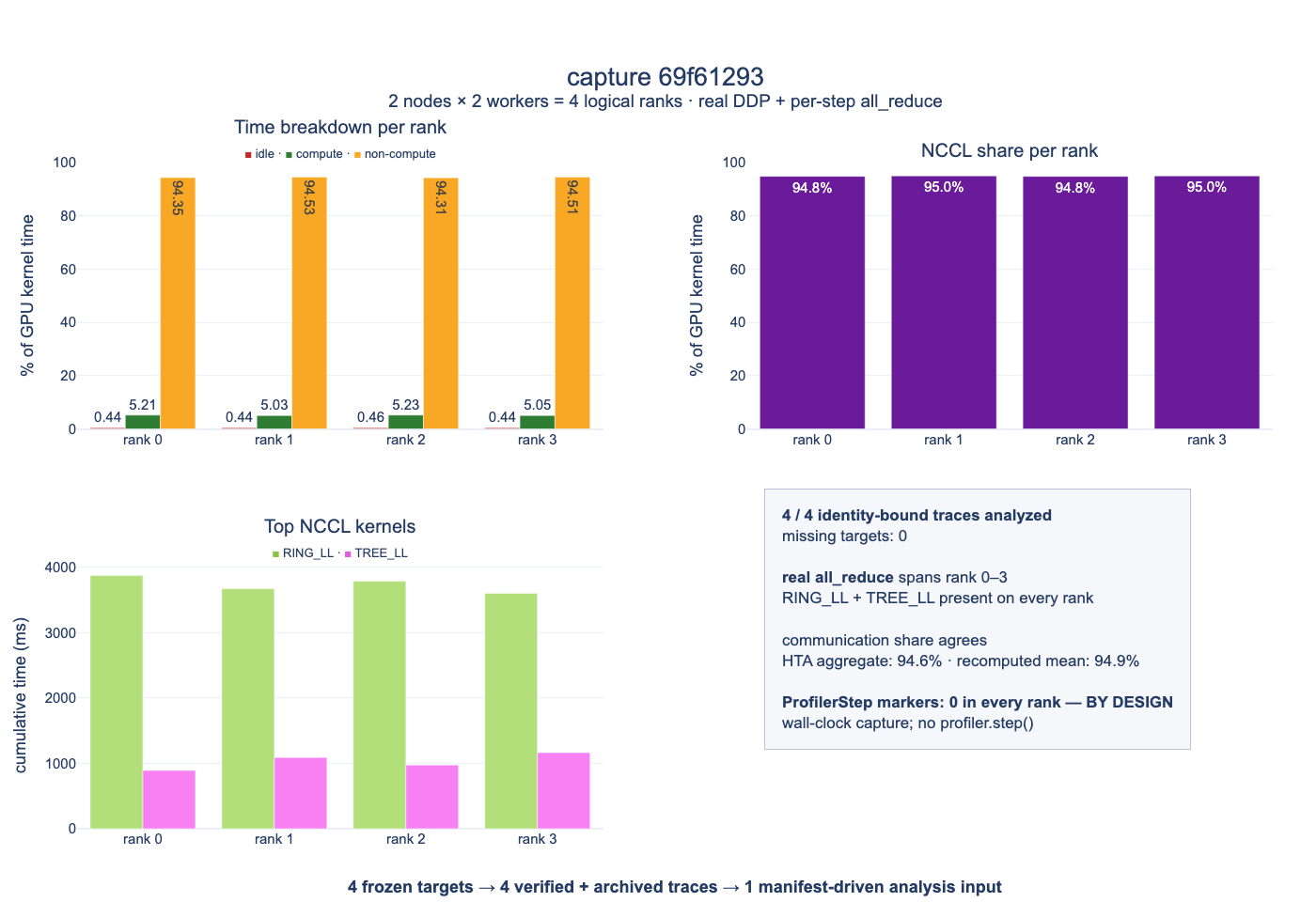
I finished by running the full pipeline on a deliberately small DDP job: two machines, two workers per training container, four ranks running a real collective. Four traces went through local observation, validation, and archival, and then an HTA Job consumed them through the manifest.

The performance ratios in this figure are not useful for workload diagnosis. The job is an intentionally synthetic communication bottleneck with very little compute. The NCCL kernel shape and roughly 1.5 GB/s effective bandwidth are much closer to Pod-network TCP behavior than NVLink.

It does not represent a real model, and it should not be used to judge whether a production training job is healthy.

The footer’s ProfilerStep markers: 0 in every rank -- BY DESIGN is also not a defect. This system provides wall-clock windows only. Iteration-scoped capture would require the training loop to call profiler.step(), which is explicitly outside this phase.

What the toy job proves is only the pipeline:

• multiple workers inside one Pod were not collapsed into one profiler target;
• ranks across nodes received the same logical capture;
• every trace was verified and archived;
• the analysis Job consumed one identity-bound, checksummed set of files through the manifest.

It is a smoke test, not a benchmark.

Closing

What I took from MAIProf was the idea that profiling should be treated as a cross-host system, not a hidden copy of an unpublished internal implementation.

The public pieces solve capture, daemon communication, and analysis. They do not answer the harder Kubernetes questions for you: who discovers the real training processes, who owns one capture, whether state survives failure, when a changing Pod set becomes fixed, and what evidence is strong enough to say a trace has actually been delivered.

The first version put those answers into one central Operator. The second version gave capture ownership back to the job, then let the node agent guard node-local facts and the manifest guard delivery facts.

It is not a line-by-line port of MAIProf. It is a different set of choices made against the same underlying problem on a different infrastructure substrate.

The hard part of on-demand profiling is not pressing the shutter. It is making every photo taken across different nodes prove that it belongs to the same shot.

The main difference between these patterns is not the tool. It is which work should remain dynamic, and which work should be materialized into a training-time artifact.

This post is a concrete case study from that design space.

It is not a Ray Data tutorial, and it is not a checklist of parameters I tuned. The real question is more basic: when GPU utilization is low, should we scale the data path, change the data layout, or stop optimizing the dataloader entirely?

My conclusion is simple:

The goal of data pipeline tuning is not to make the loader infinitely fast. It is to make the GPU stop waiting for data under the largest per-device batch or micro-batch allowed by the current training recipe.

The observations in this post come from a specific video training workload, with details abstracted where needed. The discussion focuses on a CPU decode + Ray Data streaming path. It does not cover GPU video decoding, model architecture changes, or training algorithm changes. The important part is the bottleneck reasoning process, not the absolute throughput number.

0. The one-line model

My mental model is:

training throughput = min(GPU compute / memory roofline, data supply roofline)

This is not the strict FLOPs-vs-memory-bandwidth roofline model. I am using roofline here as an engineering mental model: training throughput is bounded by both the GPU-side compute/memory ceiling and the data-supply ceiling. The lower one determines actual throughput.

So before tuning the dataloader, do not touch the dataloader.

The first step is to remove loading from the equation. Use a small controlled dataset, a controlled read path, or even fake batches if needed. Ask the GPU-side question first:

• As batch size increases, does compute start to dominate?
• Does compute become the first bottleneck, or does memory hit the limit first?
• If memory hits the limit first, what is the largest per-device batch or micro-batch allowed by the training recipe?

Only after the GPU-side workload is fixed does data_wait become meaningful. At that point, the question is:

Under the largest per-device batch or micro-batch allowed by this recipe, is the GPU worker still waiting for the next batch?

That was the tuning order in this case: first establish the GPU roofline, then raise the data roofline.

Ray Data was useful because it turned the data-supply side into an independently scalable distributed pipeline. ETL was useful because it moved repeated per-epoch work across the materialization boundary.

1. Find the GPU-side ceiling before tuning the loader

A lot of data loading work starts with low GPU utilization and immediately jumps to adding workers, increasing prefetch, or changing storage.

I think that order is risky.

Low GPU utilization can mean at least three different things:

• the batch is too small, so the GPU is not being exercised;
• the batch cannot be increased because memory hits the limit first;
• the data pipeline really is too slow, and the GPU is waiting for batches.

These have completely different fixes.

The first case needs a larger batch or heavier model-side work.
The second needs more memory, model changes, activation/memory optimization, or a different batch strategy.
Only the third is primarily a data pipeline problem.

So the first experiment I ran was a “remove the data variable” experiment. I used a small dataset, controlled the read path, and used fake batches where useful. The goal was not to measure final throughput. The goal was to establish the GPU-side load curve: as batch size increases, does forward/backward become the main component, and when does memory hit the wall?

The fake batch needs to preserve the real batch shape, dtype, device transfer path, and model input structure as much as possible. Otherwise it only measures pure model compute, not the full trainer step.

This baseline pins down the optimization target:

Reduce GPU wait under the largest per-device batch allowed by the current training recipe.

Without this baseline, data_wait is hard to interpret. A small batch can amplify data wait even when the data pipeline is not fundamentally bad. A batch that is capped by GPU memory should not be “fixed” by adding more CPU decode capacity.

2. data_wait measures GPU-facing wait, not total data pipeline cost

The profile itself is not the main point of the post. It is only a tool for answering the roofline question: is the trainer computing, or is it waiting?

The data_wait I care about is GPU-facing wait: after one training step finishes, how long does the worker block before the next batch is actually handed to the trainer?

Ray Data may still be reading from S3, decoding, collating, transferring, and prefetching in the background. If that work is overlapped with GPU compute, then it is not GPU wait.

This distinction matters. I am not trying to prove that the data pipeline has no cost. I am asking a narrower question:

Under the current maximum per-device batch or micro-batch, is the data side still making the GPU sit idle?

GPU utilization sampling is only supporting evidence. For short jobs, there may be too few samples. GPU sampling also sees only the GPU process. It does not see the CPU decode pool, the Ray object store, or operator backpressure.

For full supply-side observability, the pipeline needs cluster-level metrics such as Ray/Prometheus metrics. But for answering whether the GPU is blocked by data, worker-side data_wait is more direct.

There is one more caveat: data_wait answers a critical-path wait question, not the full end-to-end throughput story. Decode or collate cost may be hidden during steady-state steps by prefetch, while startup, tail latency, object store spilling, repartitioning, or shuffle can still stretch epoch wall-clock. Per-step profile and overall wall-clock need to be read together.

Also, CUDA kernels are submitted asynchronously. Without fixed synchronization points, some GPU work may be delayed into iterator boundaries, H2D copy, or the next step. So this profile is best used to determine whether GPU-facing wait is on the critical path, not to assign perfect absolute attribution to every substage. For that, a CUDA timeline or PyTorch profiler is needed.

3. Why Ray Data: moving the data roofline independently

The training sample in this pipeline looked roughly like this: multiple camera video frames, multiple forms of ground truth, and multiple task heads. The data lived in object storage. Downloading everything locally first was not a realistic answer. The video was stored in compressed form, so every epoch had to turn bitstreams back into pixels.

Ray Data was not useful because it magically made video decode faster. It was useful because it separated the data-supply side from the trainer-local loader:

S3 / metadata + blobs
  -> distributed read / decode / transform
  -> streaming batches with backpressure
  -> GPU trainer

This corresponds to Pattern B in my previous post: the distributed streaming DAG.

Its design contract is not “automatically faster than a pre-sharded loader.” Its design contract is that CPU-heavy data stages can scale separately from GPU-heavy training stages.

Once that separation exists, read/decode operator concurrency becomes a meaningful control. If the GPU is waiting for data, increase CPU decode concurrency. If increasing it stops helping, then the bottleneck is probably not the number of parallel slots. It may be per-sample cost, data layout, or the GPU side already reaching its ceiling.

That is the tuning taste I care about:

Identify which roofline is lower, then move the control that affects that roofline.

4. First data roofline: adding CPU helps, but it is not the root fix

The original version had a very common problem: high-resolution MP4s were decoded at runtime, while the model only needed a lower training input resolution.

The model side already had multiple task heads, but the training workers were still spending a large amount of time waiting for batches.

Increasing read_concurrency / decode concurrency was the right first move because it validated an important fact: Ray Data could move decode out of the GPU training process and raise the supply side by using an external CPU pool. As concurrency increased, wall-clock improved and GPU wait decreased.

But the experiment also showed the boundary. After a point, adding more CPU had diminishing returns.

This is where it is important not to keep tuning random parameters. If raw S3 reads are fast but the trainer is still waiting, the problem is probably not “bytes cannot be read.” The heavy work inside the ReadTask is video decode.

The first decision point was:

adding CPU helps       -> the data supply roofline was indeed too low
adding CPU plateaus    -> per-sample decode cost has become the lower bound

So Ray Data CPU scaling is a safety valve, not the final answer. It tells you where the bottleneck is, and it can buy time. But if every epoch repeatedly decodes pixels that the model will never use, the right long-term answer is not to keep buying more CPU.

5. The real leverage: moving the materialization boundary

This goes back to the core question from the previous post:

Which work should remain dynamic, and which work should be materialized into a training artifact?

Runtime decode of high-resolution video followed by resize is deterministic repeated work. If the model input resolution is already fixed, that work should not remain in the training critical path.

The biggest optimization was not changing the framework. It was ETL: re-encode the video into training resolution when building the dataset.

The decode cost is then paid once, not once per epoch, per worker, per GPU.

The benefit was order-of-magnitude. The same content encoded at training resolution is much easier to decode than “decode the full high-resolution bitstream, then downscale.” This benefit does not depend on Ray. Any loader that repeatedly decodes high-resolution video at runtime pays this tax.

This is also how I think about questions like “Ray Data vs WebDataset vs MDS vs TFRecord.” Tool choice should come after boundary choice.

First decide which processing steps should move into a training artifact. Then choose the format and execution engine that best serve that decision.

6. Bottleneck migration: once decode drops, collate appears

After ETL reduced the decode cost, GPU compute rose significantly. Work that had previously been hidden under decode started to show up.

The next bottleneck was collate. More specifically, the ground truth still existed as JSON strings inside the episode data, and runtime collate had to parse that JSON for every batch.

When decode was slow, JSON parsing looked unimportant. Once decode dropped, it became a large part of the critical path.

This is an easy mistake to make: an early profile may show a small collate percentage, but that does not mean collate is not worth optimizing. It may simply be diluted by a larger bottleneck. Roofline tuning often works this way: only after one bottleneck is fixed does the next one become eligible to appear.

The fix was the same kind of boundary movement: pre-decode structured ground truth into Arrow columns during ETL. At runtime, the pipeline only needed columnar reads and reshaping, not JSON parsing for every batch.

I prefer this over adding an in-memory LRU cache around JSON parsing. An LRU cache hides repeated cost inside each worker’s Python heap. It has unclear memory semantics and a hit-rate problem that now needs to be managed. Arrow columns turn the data into a training-time structure, reduce runtime JSON parsing and Python object construction, and fit more naturally into Ray Data’s columnar block processing.

7. Decoder optimization: useful, but only after reducing the work

Switching to a decoder such as Decord, which is better suited for video batch/random access, also helped. Its get_batch(indices) interface is useful for temporal window sampling.

This matters because a sample often needs not just one frame, but a sequence of L frames around a timestamp. Although compressed video random access is still constrained by keyframes and GOP structure, a batch/random-access decoder can avoid a lot of unnecessary frame-by-frame walking compared with a naive sequential path.

But I would still put this after ETL in the tuning story.

Decoder optimization is often a few-fold improvement. Moving high-resolution runtime decode out of the training path can be an order-of-magnitude improvement.

The tuning rule is:

first reduce the work that must be done,
then optimize the implementation of the remaining work

If the system is still decoding the full high-resolution bitstream at runtime, changing the decoder helps, but it is optimizing an operation that should not have been repeated in the first place.

8. After fixing per-device batch, check whether the data side is still worth tuning

Now we return to the GPU roofline.

After ETL, materializing ground truth into Arrow columns, and switching the decoder, I checked GPU wait again under the largest per-device batch allowed by the current training recipe. Then I swept CPU decode concurrency again.

The result was clear: a small amount of decode concurrency was already enough to feed the GPU. Adding more CPU had little marginal benefit.

That is the point where I consider the data-side question closed. Not because data_wait became exactly zero, but because:

• per-device batch / micro-batch was fixed by memory or by the training recipe;
• GPU compute had become the dominant component;
• adding data-side CPU no longer significantly reduced GPU wait;
• the remaining wait looked more like iterator/prefetch boundaries, framework synchronization, or profiling synchronization points than decode work that could be solved by more parallelism.

At this point, continuing to tune the dataloader is no longer the highest-leverage work.

To improve overall throughput further, the next questions should move to larger GPU memory, a better per-device batch / gradient accumulation strategy, more GPU workers, or more detailed tracing inside the training loop and DDP synchronization.

9. Decision rules from this tuning pass

The reusable part of this work is not a specific percentage. It is the decision order.

The same decision order explains the trade-off between eager ETL and runtime flexibility:

This is not a binary choice. A mature system often needs both: keep more dynamicity early, then move repeated work forward once the view stabilizes.

10. The order of controls in this pipeline

If I only list Ray Data API parameters, this becomes a checklist. My ordering is based on the roofline reasoning instead:

Shuffle is especially easy to misunderstand.

Ray Data streaming execution does not mean “materialize the whole dataset, then start training.” For large datasets, a shuffle strategy that requires full materialization can blow up object store pressure. A more practical approach is block/file-level reordering plus a local reservoir buffer during iteration.

This is not equivalent to a strict global random permutation, but for very large streaming training workloads, it is often a better trade-off between randomness, throughput, and resource cost.

11. Connecting back to the previous post

In the previous post, I argued that the core question in a multimodal training data pipeline is the materialization boundary:

Which stages remain dynamic, and which stages become stable training artifacts?

This case study made that framing feel even more useful.

Ray Data is a good fit for a dynamic distributed streaming DAG. It can move CPU-heavy read/decode/transform work out of the GPU trainer and scale it independently. But when a transform becomes stable and repeats every epoch, it should be moved forward.

So the conclusion is not “Ray Data wins” or “ETL wins.” A better summary is:

Ray Data gave me a control knob for moving the data-supply roofline. The roofline profile told me when to keep scaling and when to move the materialization boundary.

That is the interesting part of this kind of tuning. Good system tuning is not about turning every knob. It is about knowing which knob corresponds to the current bottleneck.

The best final state is not that the dataloader becomes infinitely fast. It is that I no longer need to keep turning the data-side CPU knob. The data path has moved back to where it should be. The remaining problems belong to the training side itself: GPU memory, compute, batch strategy, and distributed training synchronization.

Those are very different facts. A default dashboard usually shows only one of them.

I went looking for the second fact — Tensor Core activity, SM occupancy, DRAM bandwidth — inside a normal SageMaker training job. It turned into a satisfying little rabbit hole about Linux capabilities, two different ways NVIDIA exposes GPU data, and one narrow door that happens to be open on Hopper and newer GPUs.

This post is the map I wish I’d had.

The gap

nvidia-smi and W&B’s built-in system monitor both answer “is a kernel running?” They show you gpu.0.gpu utilization, memory, temperature, power, and clocks. None of that tells you how full the silicon actually is.

“Utilization 100%” can mean your SMs are saturated doing real work. It can also mean one small kernel is keeping the GPU nominally busy while the expensive units sit mostly idle.

The metrics that answer “how full” are things like:

• SM active / SM occupancy — are the streaming multiprocessors actually working, and how packed are they?
• Tensor pipe active — are you using the Tensor Cores at all?
• DRAM active — are you memory-bandwidth bound?

These are exactly the kind of signals tools like DCGM and Systalyze’s utilyze surface. So I tried to wire DCGM into a SageMaker job. It failed in a way that, once I understood it, explained everything.

Two kinds of GPU data

Here’s the thing that makes this confusing until it suddenly isn’t. “Profile my training” splits into two categories with different data paths and different privilege requirements:

This is why PyTorch Profiler’s default timeline works almost anywhere. It is the Activity API recording your kernels’ timestamps.

The moment you ask for hardware-counter data — SM activity, Tensor Core activity, memory-system activity — you are touching a global, cross-process hardware resource. NVIDIA gates that behind the driver’s performance-counter permission model. In a restricted Linux container, that effectively lands on CAP_SYS_ADMIN.

The reasoning is sound. Performance counters are a side-channel risk in multi-tenant environments, and CAP_SYS_ADMIN is a broad, dangerous capability.

So the question “can I get Tensor Core metrics in SageMaker?” reduces to a very concrete one: does my SageMaker training container have the capability needed by the normal profiling path?

The missing piece: SageMaker training containers don’t have CAP_SYS_ADMIN

I confirmed this four independent ways, because it kept feeling like surely I was just holding it wrong.

1. The error. DCGM’s dcgmi dmon for the profiling fields returns Error setting watches. Result: -29: ... requires the host engine to be running as root. The message says “root,” but the real boundary is the capability / admin counter-access path.

2. A controlled local A/B. Same image, same container. With docker run --cap-add SYS_ADMIN, the SM/Tensor fields stream. Without it, the identical -29 appears. So it is the capability, not the user id. Container “root” is not the same thing as CAP_SYS_ADMIN.

3. The API has no knob. AWS’s CreateTrainingJob API has no field for Linux capabilities or privileged mode. You can set the image, environment, resource config, VPC, entrypoint, debugger options, and so on. There is nowhere to ask SageMaker to add a container capability.

4. I measured it. I ran a probe that printed /proc/self/status. The container’s effective capabilities decode to Docker’s default set: CHOWN, DAC_OVERRIDE, FOWNER, FSETID, KILL, SETGID, SETUID, NET_BIND_SERVICE, SYS_CHROOT, and AUDIT_WRITE. CAP_SYS_ADMIN — bit 21 — is not in it. Same mask on A10G and H100.

A useful detail: in the environments I tested, this behaved like a platform-level policy, not a GPU-specific property. Even on the large exclusive instances where one job owns the physical box, the capability is still withheld. Since the capability mask was identical across the instance types I tested, the bottleneck is the way SageMaker starts the container, not the particular GPU.

So: in a stock SageMaker training job, DCGM and utilyze-style profiling counters are effectively unavailable. They require a capability that SageMaker does not expose through the training-job API.

One aside: AWS’s own GPU health-check sample can run dcgmi diag successfully on SageMaker. That briefly fooled me. But diag is a self-test path; it is not evidence that DCGM profiling counters are available.

The workaround: NVML GPM

Here’s the door that’s open.

NVIDIA’s NVML library has a feature called GPM — GPU Performance Monitoring: nvmlGpmQueryDeviceSupport, nvmlGpmSampleGet, and nvmlGpmMetricsGet.

GPM is not a full replacement for DCGM profiling. It is the path that matters for this particular problem: it exposes an overlapping class of GPU-efficiency signals — SM utilization, SM occupancy, tensor activity, DRAM bandwidth, FP16/FP32/FP64 utilization, PCIe throughput, NVLink throughput — through the NVML driver interface rather than the DCGM profiling-counter path.

And critically, in a SageMaker H100 training container with the default capability set, that NVML GPM path works without CAP_SYS_ADMIN.

There is one catch: GPM is implemented on Hopper and newer GPUs. On anything older — including A100 and A10G — nvmlGpmQueryDeviceSupport returns unsupported.

I verified both halves on actual SageMaker hardware with a tiny probe: no DCGM, no extra capability, no training loop, just NVML.

That second row is the punchline. The H100 container had the exact same capability set as the A10G one — no CAP_SYS_ADMIN — and GPM sampled fine anyway.

The point is not H100 by itself. The point is that Hopper and newer GPUs expose this NVML GPM path, while pre-Hopper GPUs do not.

So the decision tree for a SageMaker training job becomes:

Want SM / Tensor Core / DRAM utilization in a SageMaker training job?
├─ DCGM / utilyze  → need CAP_SYS_ADMIN → ✗ (not granted, can't add)
└─ NVML GPM        → accessible through the non-privileged NVML path
                     ├─ pre-Hopper (T4/A10G/A100) → unsupported → ✗
                     └─ Hopper+ (H100/H200/B200)  → ✓  ← the one open door

If your training runs on Hopper or newer hardware — and a lot of large pretraining does — you can have Tensor Core and SM-efficiency metrics in a stock SageMaker training job. Everywhere else on managed SageMaker training, you are mostly limited to the device-level metrics that W&B and nvidia-smi already give you.

Putting it together

The collection itself is refreshingly boring. It is pure NVML through pynvml: no daemon, no extra binary, no root.

You query whether the device supports GPM, take two samples a moment apart, and ask GPM for the metrics computed across that interval: SM utilization, SM occupancy, tensor activity, memory bandwidth utilization, and the rest. That’s the whole mechanism.

To make it useful for real training, run it out of band: a background thread sampling on an interval and shipping the numbers to wherever your training metrics already live. For me, that meant attaching to the same W&B run as the trainer, so the GPU-efficiency curves sit next to the loss curves.

Two practical lessons from wiring that up:

• Start it after wandb.init(), inside the training process, so you can attach to the live run. A child process can’t share that handle; a same-process background thread can.
• Fail-isolate it. A metrics collector must never slow down or crash the actual training. Sampling errors get logged and dropped, never raised.

Takeaways

• “Profile my GPU” is two questions with two privilege levels. Timeline = CUPTI Activity = no extra privilege. Efficiency/utilization counters = hardware-counter path = admin counter access / CAP_SYS_ADMIN in restricted containers. Know which one you’re asking for.
• Managed SageMaker training does not grant CAP_SYS_ADMIN, and there is no training-job API field to add it. So the DCGM / CUPTI-counter / utilyze profiling-counter family is blocked in a stock SageMaker training job.
• NVML GPM is the exception. It exposes the GPU-efficiency metrics I needed through a different, non-privileged NVML path, but only on Hopper and newer GPUs. On Hopper+, you can get Tensor Core and SM-efficiency metrics in a stock training job with nothing more than a pip dependency.
• The constraint is fundamentally about who controls the container’s capabilities. On infrastructure you control, you can add CAP_SYS_ADMIN and the normal DCGM / utilyze profiling surface opens up. On a managed platform, you ride whatever non-privileged door the vendor and driver stack leave open. On SageMaker plus NVIDIA Hopper, GPM is that door.

Kubernetes can scale Pods, but turning those Pods into the right Nodes still feels like something every DevOps or platform team has to solve by hand.

That comment stuck with me.

At first, it sounds like an implementation complaint. Maybe HPA is too limited. Maybe Cluster Autoscaler is too reactive. Maybe Karpenter needs more policy. Maybe every platform team just needs better conventions around NodePools, labels, taints, instance types, and reservations.

But after looking at the problem more carefully, I think the deeper issue is not any single autoscaler.

The issue is that Kubernetes does not have a standard way for a workload to express what kind of capacity it actually wants before the system falls back to Pending Pods as the main signal.

In other words, Kubernetes autoscaling may be missing a capacity intent layer.

That is the question I want to reason through in this post.

Over the past few years, Kubernetes autoscaling has accumulated a rich set of components and abstractions: HPA, VPA, KEDA, Cluster Autoscaler, Karpenter, Kueue, DRA, Gateway API Inference Extension, and many others. Each of them solves a real problem, and each can tell a coherent story on its own.

But if we connect these systems end to end, the operational pain my friend described becomes easier to understand.

The common autoscaling path still looks roughly like this:

HPA / workload controller / application autoscaler
  -> create or patch Pods
  -> scheduler writes PodScheduled=False, Reason=Unschedulable into Pod status
  -> Cluster Autoscaler or Karpenter observes Pending Pods
  -> node provisioning happens
  -> scheduler binds Pods to newly available Nodes

This model works well enough for many stateless services. A web service replica is usually fungible. A new Pod can handle any request after it becomes ready. Nodes are often treated as mostly interchangeable. If the cluster does not have enough capacity, creating more Pods and letting the node autoscaler react to Pending Pods is a reasonable design.

However, once the workload becomes LLM inference, Ray-based streaming, GPU batch, or stateful data processing, this chain starts to expose a more fundamental limitation.

The issue is not that HPA is too simple, or that Karpenter is not smart enough. The issue is that the downstream layers are often forced to infer too much from a low-semantic signal.

A Pending Pod mainly says:

Under the current cluster state and this Pod’s scheduling constraints, I cannot be scheduled right now.

It does not clearly say:

Why am I unschedulable? What kind of capacity do I need? How long can I wait? Can I fall back to another GPU class? Can I use Spot? Do I need warm capacity? Can I be interrupted? Is scale-down safe?

In other words, Pending Pod is a failure-after-the-fact signal. What many AI and stateful workloads need is closer to a capacity intent declared before provisioning.

HPA’s Boundary Is Not Metrics. It Is Semantics.

HPA has a deliberately narrow model. It answers one main question:

Given some observed metrics, what should the replica count of this workload be?

That abstraction was elegant in the web service era. CPU goes up, add replicas. QPS goes up, add replicas. Once new Pods become ready, a Service or ingress layer can distribute traffic to them. The scaling decision and the routing decision are relatively decoupled. Any healthy replica can usually take any request.

LLM inference is not like that.

Whether an inference replica can serve traffic is not determined merely by whether the Pod is Running. The model may still be loading. The replica may not have warmed up. KV cache locality may matter. Prefill and decode may be separated into different pools. Continuous batching may make GPU utilization look high even when the actual bottleneck is queueing, memory pressure, routing policy, or tail latency.

For LLM serving, the more relevant signals are often things like:

• request queue depth
• TTFT and TPOT percentiles
• batch slot occupancy
• prefill/decode pressure
• KV cache locality
• model load state
• routing-level backpressure
• GPU memory fragmentation or headroom

Of course, HPA can consume custom metrics. That is not the core problem.

The deeper issue is that HPA still outputs a replica count. It does not have a stable API surface to express workload properties such as:

• A new replica needs three minutes of warm-up before receiving critical traffic.
• This model must keep a minimum amount of warm capacity.
• Prefill workers and decode workers have different scaling policies.
• A cold replica without cache locality may increase tail latency in the short term.
• The bottleneck is not replica count, but queueing, routing, or downstream backpressure.
• A newly created Pod depends on a capacity policy that goes beyond fixed Pod-template constraints, such as reservation preference, fallback, capacity type, provisioning latency, or minimum lifetime.

So the limitation of HPA is not that it only looks at CPU. That is a surface-level critique. The deeper limitation is that the HPA API is not where workload capacity semantics live.

It is a replica-count controller, not a capacity intent interface.

Pending Pod Is a Lossy Interface

The Kubernetes autoscaling chain is beautifully decoupled. Workload controllers create Pods. The scheduler tries to place them. Node autoscalers observe unschedulable Pods and provision more capacity. Components communicate through Kubernetes objects rather than direct RPCs.

That decoupling is one of Kubernetes’ strengths.

But the cost is semantic loss across layers.

By the time a node provisioning layer sees the demand, the higher-level intent has often been compressed into a set of Pod-level constraints: resource requests, node selectors, affinity, tolerations, topology spread constraints, PriorityClass, labels, annotations, and maybe a few provider-specific conventions.

Those fields are useful. But they are not enough to reliably reconstruct the workload’s intent.

From a set of Pending Pods, the provisioning layer may struggle to know:

• Are these eight Pods a training gang, or eight independent online replicas?
• Must they run in the same zone, same rack, or same placement group?
• Is same-zone a hard requirement or just a preference?
• If H100 capacity is unavailable, can A100 be used as a fallback?
• Can this workload wait ten minutes for reserved capacity, or does it need on-demand capacity immediately?
• Can workers use Spot while the head or driver must use on-demand capacity?
• Should these nodes live for at least twelve hours, or can they be consolidated aggressively?
• Is this Pending state caused by real capacity shortage, quota exhaustion, reservation mismatch, or a bad scheduling constraint?
• During scale-down, which nodes are safe to drain and which would trigger expensive state reconstruction?

Some of this can be encoded today through labels, annotations, NodePools, PriorityClasses, custom CRDs, or provider-specific policies. But that is not the same thing as a stable semantic contract.

The downstream system should not have to guess.

A Pending Pod is a low-semantic-density signal centered around scheduling failure. It is good at telling the system, “Something does not fit.” It is much weaker at saying, “This is the kind of future capacity this workload is trying to acquire.”

Inference Exposes the Scale-Up Problem

LLM inference makes the scale-up gap especially obvious.

A normal stateless service often treats a replica as ready once the Pod passes readiness checks. For inference, readiness is only one part of the story. The serving stack may need to load a large model, initialize GPU memory, join a routing layer, warm up kernels, populate cache, and stabilize batching behavior.

Adding a replica can even make things worse in the short term if the routing layer sends traffic to a cold replica too early or if cache locality is destroyed.

This means there are really two layers of intent:

1. Application-level scaling intent: routing, queueing, warm-up, readiness, cache locality, prefill/decode split, and request admission.
2. Capacity-level intent: GPU class, topology, zone, reservation, capacity type, fallback policy, startup latency, lifetime, and disruption constraints.

Today these two layers are often connected indirectly. The application controller creates Pods. The scheduler fails to place some of them. The node autoscaler reacts. The cloud provider attempts provisioning. The application layer eventually learns whether the new capacity became useful.

That loop works, but it is imprecise and reactive.

For AI serving, the system often needs to know before creating arbitrary Pods:

• Do I need warm standby capacity?
• Should I provision ahead of demand?
• Should I prefer reserved capacity over on-demand?
• Is Spot acceptable for overflow only?
• Can I fall back to a cheaper GPU class?
• Should prefill and decode pools be provisioned differently?
• What is the maximum tolerable provisioning latency?

These are not simply routing decisions. They eventually affect cloud capacity provisioning. But they are also not naturally expressible as plain Pod scheduling constraints.

This is exactly the space where a capacity intent layer would help.

Streaming Workloads Expose the Scale-Down Problem

Many autoscaling discussions implicitly treat scale-up and scale-down as symmetric:

Load goes up, add capacity. Load goes down, remove capacity.

For streaming and stateful workloads, that symmetry is false.

Scale-up usually adds helpers. Scale-down removes an execution unit that may hold state, own actors, buffer data, maintain lineage, or participate in an ongoing pipeline. Removing it at the wrong time can trigger reconstruction, spilling, actor restart, backpressure, or end-to-end throughput instability.

Ray-based workloads are a useful example. Application-level actor scaling can understand pipeline bottlenecks because the application control plane knows which actors it created, what they are doing, and whether they are safe to remove. But at the cluster level, node autoscaling typically sees much lower-level signals: resource requests, utilization, idleness, Pod disruption budgets, taints, and node-level constraints.

Ray Data makes this distinction especially concrete. Its application-level execution can scale actor pools based on pipeline pressure and operator bottlenecks, because that logic lives close to the data execution graph. But cluster-level scale-down is necessarily more conservative. A worker node should only be reclaimed after the application has stopped using it and the node becomes idle. In other words, Ray Data can be relatively proactive about application-level scale-up, while cluster-level scale-down is closer to passive reclamation after the workload has made capacity safe to remove.

That distinction is the important part. Safe scale-down is not just a utilization problem. It is an application-state problem.

A node provisioning layer usually cannot know:

• whether a worker currently holds important actor state
• whether deleting a Pod will trigger expensive object reconstruction
• whether low CPU means idle or blocked by downstream backpressure
• whether a streaming pipeline is in a safe drain point
• whether a node is safe to consolidate now or should be preserved

For these workloads, the intent is not merely min/max replicas. The workload needs to express properties like:

• This worker group may scale up automatically, but scale-down must be application-drain-only.
• These nodes may be consolidated; those nodes must not be consolidated.
• These Pods are on the critical path and should not be randomly disrupted by infrastructure-level optimization.
• Spot is acceptable for buffer capacity, but not for baseline capacity.
• Drain must complete before scale-down; if the drain timeout fails, keep the node.

These semantics do not belong entirely to HPA. They also do not belong entirely to kube-scheduler. They need to flow across the boundary between workload control and node provisioning.

DRA Points in the Right Direction

Dynamic Resource Allocation is not a node autoscaler. It solves a different problem: how workloads declare, select, allocate, and prepare devices that exist in the cluster.

But DRA is interesting beyond GPUs or device plugins. It points toward a more explicit resource model.

Instead of reducing device demand to something like:

resources:
  limits:
    nvidia.com/gpu: 1

DRA introduces a richer model. DeviceClass describes categories of devices. ResourceClaim expresses a workload’s resource request. ResourceSlice represents available device inventory. The scheduler can reason about claims and constraints. The driver participates in preparing and unpreparing resources on the node. Status records the allocation result.

The important shift is this:

A resource is no longer just an integer. It becomes an object with class, attributes, constraints, allocation result, and lifecycle.

Node provisioning faces a similar problem, but at a harder layer.

DRA mostly operates over devices and nodes that already exist. Node autoscaling often deals with cloud capacity that does not exist yet. The candidate space is much larger:

instance type
x zone
x capacity type
x reservation
x quota
x price
x startup latency
x topology / placement constraints

Placement group is not quite the same type of dimension as instance type or zone. It is more like a supply-side topology constraint. Quota is not inventory. Reservation is not ordinary capacity. Spot has interruption risk. Capacity block has time boundaries. Startup latency matters. Price changes the optimization objective.

Cloud providers also do not expose complete real-time inventory to Kubernetes. A failed CreateFleet or RunInstances call is not an exceptional corner case; it is often part of the solving process. Fallback, reservation selection, quota, placement, capacity type, and startup latency are all provider-side concerns.

So node autoscaling should not copy DRA directly.

But it can borrow DRA’s schema philosophy:

• claim-based requests
• class-based policy
• explicit constraints
• provider-specific solving
• allocation status
• lifecycle-aware cleanup
• understandable failure reasons

DRA does not solve cloud capacity provisioning. But it shows why richer resource semantics matter once resources stop being fungible integers.

The Missing Layer: Capacity Intent

If I had to give the missing piece a name, I would call it Capacity Intent, not Autoscale Policy.

An autoscale policy usually says:

Under these metrics, change the replica count this way.

Capacity intent says something different:

This workload needs a certain kind of capacity, and here is how that capacity may be supplied, substituted, reserved, disrupted, and eventually released.

A hypothetical object might look like this:

apiVersion: capacity.k8s.io/v1alpha1
kind: CapacityClaim
metadata:
  name: llama-decode-capacity
spec:
  workloadType: inference

  podSets:
    - name: decode-workers
      count: 8
      templateRef: decode-worker-template

  latency:
    maxProvisioningLatency: 5m
    warmCapacityRequired: true

  topology:
    locality: same-zone
    placementGroup: preferred

  capacityPolicy:
    capacityTypes:
      - reserved
      - on-demand
    spotAllowed: false
    fallback:
      - gpuClass: h100
      - gpuClass: a100

  disruption:
    minLifetime: 12h
    consolidationAllowed: false
    scaleDownPolicy: application-drain-only

This object does not have to be called CapacityClaim. It may not even need to become a Kubernetes core API. The exact API shape is less important than the missing semantic contract.

The contract should allow the workload to express:

• what type of capacity it needs
• whether the capacity must be warm
• how long provisioning may take
• what topology constraints matter
• which capacity types are acceptable
• whether fallback is allowed
• whether the workload is interruptible
• how scale-down must be coordinated
• how long the capacity should live
• what failure reasons should be reported back

With this layer, the flow becomes different:

Workload declares capacity intent
  -> admission checks quota, fairness, and policy
  -> provisioning layer solves for node capacity
  -> cloud provider attempts allocation
  -> status reports selected capacity or failure reason
  -> scheduler binds Pods to nodes that satisfy the intent

The key change is that capacity is declared before the system relies on scheduling failure as the primary signal.

That is a very different model from:

Create Pods first
  -> let them fail scheduling
  -> infer demand from failure
  -> provision nodes

For simple services, the current model is fine. For AI and stateful workloads, it often forces too much information to be reconstructed too late.

ProvisioningRequest Is Already Pointing in This Direction

There are already signs that the Kubernetes ecosystem is moving toward this idea.

Cluster Autoscaler’s ProvisioningRequest, and Kueue’s integration with it through AdmissionCheck, is one example. The important idea is not that ProvisioningRequest solves every workload category. It does not.

The important idea is that capacity availability can be checked before workload admission instead of being discovered only after Pods become Pending.

That matters.

For batch workloads, this is a natural fit. A job may need a whole group of Pods admitted together. It may not make sense to create all Pods, let them sit Pending, and then hope the autoscaler guesses the group-level intent correctly. By moving capacity checks into admission, the system can reason about the workload as a unit.

But this is still not the full capacity intent layer for inference, streaming, or stateful AI workloads.

It does not fully express:

• warm capacity
• pre-provisioning
• fallback between GPU classes
• reservation lifecycle
• Spot as overflow capacity only
• application-drain-only scale-down
• cache locality
• long-running cluster semantics
• workload-specific disruption constraints

There is also an important caveat: the practical value of this mechanism depends on the autoscaler and cloud provider implementation behind it. Moving the request earlier in the admission path is useful, but the API alone does not guarantee that the provider has enough inventory visibility, supports the relevant capacity classes, can reason about reservations, or can return rich fallback and failure status.

So ProvisioningRequest is best understood as an important signal in the right direction: capacity should become explicit earlier in the control loop.

It is a bridge toward capacity intent, not proof that the full interface already exists.

Cloud Providers Need to Participate in the Solving Loop

A common platform instinct is to solve everything inside Kubernetes.

For node provisioning, that instinct has limits.

Many critical facts only exist on the cloud provider side:

• which zone currently has a certain GPU instance type
• whether a reservation can satisfy the request
• whether a capacity block is usable
• whether a placement group can still fit the requested nodes
• whether account quota is sufficient
• whether Spot is available and at what risk profile
• how long a certain instance family usually takes to start
• whether fallback to another instance type changes cost and performance too much

Kubernetes should not pretend to have perfect global inventory.

A more realistic role for Kubernetes is to standardize the upper-layer intent, then delegate provider-specific solving to the provisioning implementation. The provider integration can solve within NodePool constraints and translate intent into instance types, zones, capacity types, reservations, NodeClaims, or cloud-specific allocation requests.

Then it should report back through status conditions:

• capacity unavailable
• quota exceeded
• reservation mismatch
• fallback selected
• provisioning in progress
• partially fulfilled
• expired
• interrupted
• drain required
• consolidation blocked

This feedback loop is as important as the initial request.

Without explicit status, the workload layer only sees that Pods are Pending, nodes are missing, or replicas are not useful yet. That is too opaque for complex AI systems.

Karpenter already moves beyond traditional static node groups by dynamically selecting instance types and creating capacity within the boundaries of NodePools and provider-specific NodeClasses. That is a major improvement over older node group-centric models.

But Karpenter still primarily reasons from Pods and their scheduling constraints. The next step is not merely to make node autoscalers more clever at reading Pending Pods. The next step is to give them better intent to work with.

This Is Not a Universal Autoscaler

There is an easy trap here.

Once we say HPA is not enough and Pending Pod is too lossy, it is tempting to propose a universal autoscaler that manages online services, LLM inference, training, batch, streaming, and stateful data processing through one giant control plane.

I do not think that is the right answer.

These workloads have different scaling semantics.

For ordinary online services, scaling usually means adding fungible replicas.

For LLM inference, scaling is a joint problem across routing, queueing, batching, GPU memory, cache locality, model loading, warm capacity, and capacity provisioning.

For distributed training, the main problem is often not autoscaling at all. It is admission, gang scheduling, topology, failure recovery, checkpointing, quota, and preemption.

For streaming, scale-up and scale-down are not symmetric. Scale-down has to respect application state, drain semantics, and pipeline stability.

Trying to hide all of that behind one universal autoscaler would likely create another overloaded abstraction.

A better direction is to let each workload keep its own control plane:

• HPA can continue to serve ordinary replica scaling.
• KEDA can continue to connect event sources to replica scaling.
• Kueue can continue to handle batch admission and quota.
• DRA can continue to express device allocation.
• Karpenter and cloud-provider integrations can continue to handle node provisioning.
• Inference gateways and serving controllers can continue to own request routing, warm-up, and traffic admission.
• Ray, Spark, Flink, and similar systems can continue to manage their own application-level execution semantics.

The missing piece is not one controller to replace all of them.

The missing piece is a clearer contract between them.

That contract should let the workload say:

Here is the kind of capacity I need, the constraints under which it is useful, and the lifecycle rules under which it may be changed.

And it should let the provisioning layer say:

Here is what I can allocate, what fallback I selected, why I failed, and what disruption guarantees I can or cannot provide.

That is what I mean by a capacity intent layer.

Why This Matters More for AI Infrastructure

This problem existed before AI workloads became popular. Stateful services, distributed data processing, and batch systems have always stretched the Kubernetes scheduling model.

But AI infrastructure makes the issue much more visible.

First, the resources are less fungible. An H100 is not just a bigger CPU. GPU class, memory size, interconnect, topology, MIG configuration, driver version, and placement all matter.

Second, startup cost is higher. Loading a large model, warming kernels, joining a distributed runtime, or restoring state can take meaningful time.

Third, routing and capacity are tightly coupled. A new inference replica is not automatically useful. It must be integrated into request routing, batching, cache, and admission control.

Fourth, cloud capacity is uncertain. GPU supply, reservations, capacity blocks, quota, and Spot availability are all part of the operational reality.

Fifth, disruption is expensive. Removing the wrong node may not just restart a stateless Pod. It may disrupt actors, invalidate cache, trigger object reconstruction, or destabilize a pipeline.

These properties do not fit cleanly into a world where node provisioning mostly learns demand from unschedulable Pods.

AI infrastructure needs a stronger language for capacity.

Conclusion

This brings me back to my friend’s complaint.

The reason Kubernetes autoscaling often feels like it still needs a lot of hand-built DevOps logic is not simply that the autoscalers are immature or that the metrics are not good enough.

A deeper reason is that workload intent is lost as it crosses layers.

HPA sees metrics and outputs replica count.

The scheduler sees Pods and constraints.

Karpenter or Cluster Autoscaler sees Pending Pods.

The cloud provider sees instance provisioning requests.

Each layer has local facts, but there is no standard way to express the workload’s capacity properties across the whole path.

Of course, many fields can be encoded today in Pod templates, ResourceClaims, PriorityClasses, topology spread constraints, annotations, custom controllers, NodePools, or provider-specific CRDs. The problem is not that expression is impossible. The problem is that the expression is scattered, implicit, and often reconstructed by convention.

Scattered expression is not a stable interface.

DRA already shows one important lesson on the device side: when resources become complex, an integer request is not enough. The system needs explicit resource attributes, constraints, allocation results, and lifecycle.

Node autoscaling needs a similar evolution, not by copying DRA directly, but by bringing the same philosophy to cloud capacity provisioning.

So the next step for Kubernetes autoscaling may not be to observe Pending Pods more cleverly.

It may be to make the system rely on Pending Pods less.

For simple workloads, scheduling failure can remain a reasonable trigger.

For AI and stateful workloads, capacity should become an explicit intent before every platform team is forced to encode the missing semantics by hand.

This post is my attempt to make that observation useful rather than pedantic. I want to sort these systems into a few workflow families, using representative examples rather than attempting an exhaustive product comparison. Airflow, Argo, KFP, Flyte, Dify, and ADK are useful because each makes a different execution contract visible. The point is not that these are the only workflow systems worth discussing, or that every deployment of each system behaves exactly the same way. The point is that the word workflow hides several very different architectural choices.

The two axes I find most useful are:

1. What is the scheduling unit?
2. When does the DAG become real?

A third question follows from those two: what kind of durability contract does the system provide?

These questions explain more than feature checklists. A workflow step may mean a function call inside one Python process, a task picked up by a long-running worker, or a new Pod created on a Kubernetes cluster. A DAG may be a Python file parsed by a scheduler, a compiled intermediate representation, a registered entity in a control plane, a Kubernetes custom resource, or an in-process graph traversed during a request. These are not small implementation differences. They define latency, isolation, retry semantics, operational complexity, and the kinds of workloads the system naturally fits.

Here is the simplified map before going into details:

This table is intentionally rough. Real systems have plugins, executors, backends, and deployment modes that can shift details. But the table captures the design center of each family. When teams skip this layer and compare all of them under the single label “workflow,” they often end up evaluating the wrong thing.

The two axes

Axis 1: scheduling unit

When the engine “runs a step,” what does that mean physically?

Is it a function call inside the same Python process? A task picked up by a long-running worker? A new Pod created on a Kubernetes cluster? A container launched by a pipeline backend? These choices have very different latency floors, isolation boundaries, and failure modes.

Most workflow systems have a design center on this axis. Some have multiple executors or deployment modes, but the design center still matters because it shapes the operational model users inherit.

Axis 2: DAG plasticity

When is the DAG “real”?

Is it written in a file at deploy time and parsed by a scheduler? Is it compiled at registration time into an intermediate representation? Is it submitted as a Kubernetes custom resource? Is it traversed inside a single request, possibly while an LLM decides the next action?

“Static at deploy time” and “dynamic per request” are not merely points on a spectrum. They imply different control-plane assumptions. A scheduler that can backfill yesterday’s failed ETL run is solving a different problem from an agent graph that streams tokens back to a user in one request.

Consequence: durability contract

The scheduling unit and DAG materialization point usually determine the durability contract.

Airflow cares about scheduled task instances, retry, backfill, and operator visibility. Argo cares about Kubernetes resources, Pod lifecycle, artifact passing, and workflow status. KFP and Flyte care about reproducible pipeline runs and containerized tasks. Agent workflows care about low-latency orchestration inside an interactive request.

A system can sometimes be extended beyond its design center. But if the durability contract does not match the workload, the integration tends to feel unnatural.

The ETL model: Airflow and the self-managed worker tradition

Airflow is the oldest system in this discussion, and for a long time it was the workflow engine in many data teams: the default answer when people meant scheduled ETL, dependency management, retries, and backfills.

Airflow’s architecture is organized around a scheduler, task instances, metadata state, and a configured executor. The scheduler decides when a task is ready; the executor determines how the task is physically run. In a historically common production setup, CeleryExecutor dispatches tasks to long-running Celery workers. In other deployments, LocalExecutor, KubernetesExecutor, or hybrid executors can change the physical execution backend.

So the careful statement is not that Airflow can only run tasks on Airflow-owned workers. It cannot; KubernetesExecutor exists and launches Pods. The more useful statement is that Airflow’s design center is an Airflow task instance managed by the Airflow scheduler/executor model, rather than a Kubernetes-native Workflow custom resource.

DAG plasticity is also on the static side. A DAG is usually a Python file in a DAG folder; the scheduler parses it and creates task instances according to schedules and dependencies. Airflow 2.x introduced dynamic task mapping, which is useful for runtime fan-out over collections, but it does not turn Airflow into a per-request dynamic agent runtime.

This is not a criticism of Airflow. Airflow is well suited to what it was originally built for: scheduled batch workflows where individual tasks may take minutes or hours, reliability matters more than per-hop latency, and backfill is a first-class operational requirement.

The mismatch appears when Airflow is pressed into workloads with different contracts: tight ML training loops, interactive serving paths, or LLM agent orchestration where a few seconds of orchestration latency is already too much.

The Kubernetes-native model: from worker pool to Pod

Once Kubernetes became the substrate for many ML and data platforms, a different question became natural:

If Kubernetes already schedules Pods with quotas, node selectors, topology, and resource constraints, why should a workflow system maintain its own worker pool inside the cluster?

Argo Workflows is a representative answer to that question.

In Argo, the design center is Kubernetes-native execution. A workflow is a Kubernetes custom resource. The controller reconciles that resource. Each step is typically represented by a Pod or Kubernetes execution primitive, and kube-scheduler decides where it lands.

This shifts the workflow engine out of the placement business. Argo defines workflow structure, dependencies, retries, parameters, and artifacts; Kubernetes handles Pod placement. That distinction matters. If a platform’s real problem is GPU quota, gang scheduling, topology-aware placement, or cluster-level admission control, changing workflow engines alone is unlikely to solve it. Those concerns sit closer to the Kubernetes scheduler, resource admission, Kueue, Volcano, or platform-specific placement logic.

Argo’s DAG also lives outside the user container. A workflow is submitted as a custom resource. Because steps are separate Pods, artifact passing becomes the natural communication pattern. A producing step writes declared output artifacts; the workflow system stores them in a configured artifact repository; a downstream step reads them as inputs.

This is strong for reproducibility, retry, and isolation. It is not the same as an in-memory streaming dataflow engine like Spark or Flink. Both may draw DAGs, but the data movement contract is different.

That distinction explains a common platform confusion: a workflow DAG is not automatically a data-processing DAG. Argo can orchestrate steps that process data. It does not, by itself, become a high-throughput distributed data engine with shuffle, pipelined execution, and memory-aware data movement.

Pythonic ML pipelines on top of workflow backends

Raw YAML is not the interface most ML engineers want. That created a second layer of systems: Pythonic ML pipeline authoring systems that compile or register workflows onto a backend execution system.

Kubeflow Pipelines and Flyte are representative examples, but they choose noticeably different shapes.

Kubeflow Pipelines: Python as an authoring and compilation layer

In the classic standalone KFP v1 deployment, Kubeflow Pipelines used Argo Workflows as the workflow engine. That does not mean every modern KFP-conformant backend is Argo. KFP v2’s IR and conformant-backend model explicitly decouple authoring from a single execution backend.

The more durable architectural point is this: KFP treats Python primarily as an authoring and compilation layer.

You write @dsl.component and @dsl.pipeline functions in Python. The SDK compiles the pipeline into an intermediate representation. At run creation time, the backend turns that representation into whatever execution format it supports. In the Argo-backed deployment, that means Argo Workflow resources. In other backends, it may mean something else.

The important property is that the Python pipeline definition is not the runtime process executing every step. Task code is packaged into containers. The pipeline topology has already been compiled into a backend-consumable form. Main and task are not running in the same Python execution context.

This makes KFP feel different from both Airflow and in-process agent frameworks. It is not a scheduler parsing DAG files forever, and it is not a request-time control loop. It is an ML pipeline authoring layer with a compiled execution representation.

Flyte: Python as a registration-time entity

Flyte is another route to Pythonic ML/data workflows, but it has a different shape.

Flyte makes tasks and workflows Python-decorated entities that are registered with the control plane. At registration time, Flyte serializes task definitions, workflow structure, image references, interface definitions, and other execution metadata into a registered entity.

This gives Flyte a strong type-aware, reproducible, control-plane-centric model. It also means SDK ergonomics matter a lot. If image dependencies, runtime configuration, copied source files, Spark configuration, and workflow structure are colocated in decorators and registration metadata, ordinary operational changes can enter the image or registration loop.

That is not an inherent limitation of Flyte. Flyte provides mechanisms such as reusable container images, ContainerTask, fast registration, and other ways to separate orchestration from image lifecycle. A disciplined team can keep those layers clean.

The point is narrower: Flyte’s design center makes Python a registration-time source of truth, not just a YAML generator and not an in-process request runtime. That gives it a different coupling surface from KFP. KFP tends to make Python disappear into compiled IR; Flyte tends to preserve Python-defined entities as registered control-plane objects.

That difference matters when thinking about iteration loops, image lifecycle, and the boundary between business logic, orchestration metadata, and runtime environment.

Workflow is not ML pipeline, and ML pipeline is not MLOps

This is the section I think many ML infrastructure discussions skip too quickly.

A pipeline engine solves one slice of the problem: how steps connect to each other and run in order. That is useful, but it is not the whole of MLOps.

MLOps, if the term means anything operationally, includes more than step orchestration:

• experiment tracking
• run comparison
• model registry
• lineage from data and code to model artifact
• distributed training job integration
• serving and deployment integration
• notebook and development environments
• data and artifact versioning
• reproducible runtime environments

KFP runs pipelines. Flyte runs workflows. Argo runs workflows. Airflow runs scheduled DAGs. None of these, on its own, is a complete MLOps platform.

Kubeflow as a broader distribution is closer to a platform because it includes components beyond KFP: training operators, Katib, KServe, notebooks, model registry work, and integrations around the ML lifecycle. But KFP-the-pipeline-engine and Kubeflow-the-ML-platform are not the same thing.

This distinction matters because teams often install a pipeline engine and assume they have installed MLOps. They have not. They have installed orchestration. They still need to decide how experiments are tracked, how models are registered, how training jobs report metrics, how lineage is preserved, how artifacts are promoted, and how serving is connected.

Installing a pipeline engine and calling it MLOps is a bit like installing make and calling it CI/CD.

The agent model: the scheduling unit shrinks back into the process

The newest source of confusion is the agent ecosystem adopting the word “workflow.”

This is not wrong exactly. Agent frameworks do orchestrate steps. But their execution contract is very different from Airflow, Argo, KFP, or Flyte.

Google ADK’s older Workflow Agents, such as SequentialAgent, ParallelAgent, and LoopAgent, were deterministic templates for sub-agent execution. Current ADK documentation says these template workflows have been superseded by graph-based and dynamic workflows starting in ADK 2.0. That changes the API surface and flexibility story, but it does not make ADK equivalent to Airflow or Argo.

The design center is still low-latency orchestration of agents, tools, and graph nodes inside an application/request context. A ParallelAgent-style fan-out is closer to coroutine concurrency over sub-agents than to Kubernetes scheduling. It is useful for parallel LLM/tool calls. It is not the same thing as launching independent Pods across a cluster with durable artifact lineage.

Dify Workflows sit in a similar broad family from an architecture perspective. Dify may persist workflow runs and use background workers for parts of the application, but it should not be confused with a durable batch scheduler like Airflow or a Kubernetes-native workflow controller like Argo. Its design center is application-level orchestration for LLM apps: nodes, variables, prompts, tools, model calls, and user-facing execution.

This explains the practical mismatch.

Putting an LLM agent loop on Airflow introduces a scheduler and task-instance model into a path that wants low-latency token streaming. Putting a daily ETL job on an agent workflow framework gives up the operational contract that ETL teams usually need: backfill, long-running scheduler state, retry policy, historical observability, and failure handling at 3 AM.

Both systems may call the thing a workflow. They are not solving the same problem.

A more useful comparison

The systems become easier to compare if we stop asking which one is the best workflow engine and instead ask what execution contract each one gives us.

This is still simplified, but it is much more useful than a flat feature comparison.

A few examples follow directly:

• If you need backfill and scheduled dependency management, start with Airflow-style assumptions.
• If you need Pod-level isolation and Kubernetes-native execution, start with Argo-style assumptions.
• If you need reproducible containerized ML pipelines with Python authoring, start with KFP/Flyte-style assumptions.
• If you need low-latency LLM application control flow, start with agent-workflow assumptions.

A system can sometimes be stretched outside its design center, but the stretch should be explicit. Otherwise the team mistakes a naming overlap for architectural compatibility.

A small test before choosing anything called a workflow

Before committing to any workflow system, I would ask these questions in order.

1. What is the scheduling unit?

A worker process? A Kubernetes Pod? A containerized backend task? An in-process function call? A coroutine? A sub-agent?

This tells you the latency floor, isolation model, resource boundary, and most of the operational shape.

2. When does the DAG become real?

A Python file parsed by a scheduler? A YAML custom resource submitted to Kubernetes? A compiled IR? A registered entity? A graph traversed inside a request?

This tells you how dynamic the system really is, and where the control plane lives.

3. What durability contract do you need?

Do you need retry and backfill? Artifact lineage? Kubernetes-native status? ML pipeline run metadata? Or do you mostly need request-local orchestration and streaming?

Durability is not a feature checkbox. It is part of the workload contract.

4. Are you actually asking for workflow, ML pipeline, or MLOps?

A workflow engine runs ordered steps. An ML pipeline gives ML-oriented authoring and reproducibility around those steps. MLOps includes the broader lifecycle: experiments, model registry, deployment, lineage, serving, and governance.

If the real problem is MLOps, choosing a workflow engine is only one part of the answer.

Closing thought

The label “workflow” is fine as marketing, but weak as an architecture tool.

It does not tell you what the scheduling unit is. It does not tell you when the DAG becomes real. It does not tell you what durability contract the system provides. It does not tell you whether the system is built for scheduled ETL, Kubernetes-native batch execution, reproducible ML pipelines, or interactive agent applications.

So I would not start with:

Which workflow engine should we use?

I would start with:

What execution contract does this workload need?

Once that is clear, the comparison becomes much less confusing. Airflow, Argo, KFP, Flyte, Dify, and ADK are not just competing products under one label. They are representative points in different workflow families. Treating them that way makes the design discussion more honest.

That sounds close to multi-cloud GPU scheduling.

But it is not the same problem.

MultiKueue is useful Kubernetes-native plumbing for dispatching workloads from a manager cluster to worker clusters. That is a real capability. It lets users submit jobs through one control point while executing them on remote Kubernetes clusters. But remote dispatch should not be confused with GPU placement.

For GPU workloads, the hard question is not merely:

Which cluster should receive this Kubernetes Job?

The harder question is:

Which resource pool can actually run this workload with the right GPU topology, quota, data locality, cost boundary, tenant policy, and recovery semantics?

Those are different problems.

What MultiKueue Actually Does

MultiKueue’s core model is straightforward. A manager cluster connects to one or more worker clusters. The manager creates and monitors remote Workloads or Jobs on worker clusters and synchronizes status back to the local objects. Worker clusters still behave like standalone Kueue clusters.

By default, MultiKueue uses the AllAtOnce dispatching mode: once the manager-side Workload obtains a QuotaReservation, the Workload is copied to all available worker clusters. The first worker cluster that admits the remote Workload becomes the selected cluster; the manager then deletes the remote Workloads from the other clusters and creates the corresponding Job in the selected worker cluster.

MultiKueue also supports Incremental and External dispatcher modes. Incremental nominates worker clusters gradually in rounds, while External delegates worker-cluster nomination to a custom controller. These modes can narrow or customize the candidate set, but they do not change the core boundary: the manager dispatches after its own quota reservation, and the actual worker-side admission result is resolved after dispatch.

In the right scope, this is useful. If an organization owns several Kubernetes clusters and wants a centralized submission path for Kubernetes-native batch workloads, MultiKueue provides a reasonable mechanism.

But that is still a dispatch mechanism.

It does not automatically solve the full placement problem for GPU workloads across clouds, regions, reservations, pricing models, topology constraints, and data boundaries.

This distinction matters because GPU scheduling is not only about moving a Kubernetes object from one API server to another. It is about deciding where a high-value, topology-sensitive, data-sensitive workload should run.

The Awkward Middle: Manager-Side Quota Approximation

The most awkward part of MultiKueue’s model is the manager-side quota approximation.

The official documentation states that the quota configured in the manager cluster should ideally equal the total quota available across all worker clusters. If the manager quota is significantly lower, worker clusters may remain underutilized. If the manager quota is significantly higher, the manager may dispatch and monitor workloads that are unlikely to be admitted in the worker clusters.

That is the core tension.

If the manager-side quota is conservative, expensive GPUs may sit idle in worker clusters while jobs wait in the manager queue.

If the manager-side quota is optimistic, the manager may send workloads to worker clusters that cannot actually admit them.

Either way, the manager-side quota is not the source of truth. It is a model.

For ordinary batch workloads, this kind of approximation may be acceptable. For GPU workloads, especially expensive multi-GPU or multi-node training jobs, the cost of a weak placement decision is much higher.

A GPU scheduler cannot only ask:

Is there some quota somewhere behind a worker cluster?

It often needs to know:

Which GPU model is available?
Is it H100, H200, A100, L40S, or something else?
Is it PCIe, SXM, NVL, or a full HGX-style node?
Is the workload single-node or multi-node?
Is the required network available?
Is this capacity reserved, on-demand, or preemptible?
Is the data nearby?
Is cross-cloud or cross-region egress allowed?
Which tenant owns the budget?
What is the queue pressure in the target pool?
Can this job recover if the node disappears?

These signals are not just implementation details. They are the placement decision.

Dispatch Is Not Placement

This is the claim boundary that often gets blurred.

Dispatch means:

Take this workload and submit it to a selected worker cluster.

Placement means:

Decide which resource pool should run this workload,
given real capacity, queue pressure, GPU topology, data locality,
tenant policy, cost, priority, and failure recovery requirements.

MultiKueue helps with the first problem.

It does not, by itself, own the second problem.

This difference is especially important for GPU infrastructure because GPU resources are not fungible in the same way as generic CPU capacity. Eight H100s in one cloud region are not necessarily equivalent to eight H100s in another region or provider. The instance shape, local GPU interconnect, inter-node network, reservation status, storage path, data locality, and operational boundary all matter.

Treating all of that as a remote-cluster dispatch problem hides the hardest part of the system behind a Kubernetes-native abstraction.

Kueue’s Model Is Powerful, But Its Strength Has a Boundary

Kueue’s internal model is powerful inside a Kubernetes control domain.

A ClusterQueue governs a resource pool and defines quotas, usage limits, and fair-sharing rules across multiple ClusterQueues. It can manage resources such as pods, CPU, memory, and hardware accelerators.

A ResourceFlavor represents resource variations and associates them with nodes through labels, taints, and tolerations.

A Cohort lets ClusterQueues share quota with each other, allowing unused quota to be borrowed within the same sharing structure.

This is a good model for Kubernetes-native quota and admission control.

The problem starts when this model is over-generalized into enterprise multi-cloud GPU scheduling.

A department is a business concept.

A cloud GPU pool is a technical and economic entitlement.

A GPU placement decision is a combination of capacity, topology, cost, policy, and data constraints.

Those concepts do not always map cleanly into a single queue/cohort/flavor graph.

Inside a stable Kubernetes GPU pool, Kueue’s model can be a strong fit.

Across dynamic cloud GPU capacity, the model becomes much harder to reason about.

The Fork in the Road

MultiKueue faces a fundamental fork.

If it does not know real worker-side quota, queue pressure, GPU topology, data locality, tenant budget, and cost constraints before dispatch, then it can only make a best-effort remote submission.

If it does know all of those signals before dispatch, then the real placement decision is already being made somewhere else. At that point, MultiKueue becomes one execution path, not the top-level scheduling abstraction.

This is why the manager-side quota approximation is not a minor detail. It reveals the deeper issue: MultiKueue is not designed to be the full source of truth for multi-cloud GPU placement.

It can move jobs across clusters.

But moving jobs is not the same as deciding where expensive GPU workloads should run.

Where MultiKueue Fits

The point is not that MultiKueue is useless.

It is useful for what it is:

Kubernetes-native multi-cluster job dispatch.

It is a reasonable fit when:

The organization owns multiple Kubernetes clusters.
The clusters are relatively stable.
The workloads are Kubernetes-native.
The main goal is centralized submission and remote execution.
The placement policy is simple enough to be approximated at the manager.

But it should not be over-sold as:

A complete enterprise multi-cloud GPU scheduler.

That broader problem requires placement decisions based on signals that go beyond remote Kubernetes object creation.

Conclusion

MultiKueue solves dispatch, not multi-cloud GPU placement.

That distinction matters.

For GPU workloads, the hard part is not simply sending a Job to another cluster. The hard part is deciding which resource pool should run the workload in the first place, given GPU topology, quota, queue pressure, data locality, tenant policy, cost, and recovery requirements.

MultiKueue is useful Kubernetes-native plumbing. But treating it as the center of a multi-cloud GPU scheduling architecture risks overestimating what remote dispatch can solve.

The right claim boundary is simple:

MultiKueue can help dispatch Kubernetes workloads across clusters.
It should not be confused with a full multi-cloud GPU placement system.

References

• Kueue overview
• MultiKueue concept
• ClusterQueue concept
• ResourceFlavor concept
• Cohort concept

When I look at large-scale multimodal training data systems, I keep seeing the same confusion: people compare tools before agreeing on which lifecycle stage they are optimizing. A data curation system, a storage layout, a training-time DataLoader, and a cache strategy are related, but they are not the same layer.

So this post is not a benchmark report, and it is not a universal architecture recommendation. It is a personal reasoning framework: how I currently think about the design space, what patterns seem to appear repeatedly, and where I think the real trade-offs are.

The core question I keep coming back to is:

At which point in the data lifecycle should a pipeline stop being dynamic and become a stable training artifact?

That boundary determines how much flexibility the system keeps, how much throughput the training loop can get, and how expensive dataset evolution becomes.

1. The real problem: data lifecycle, not just data loading

A multimodal training pipeline usually has more stages than the final DataLoader.

A simplified lifecycle looks like this:

raw recording
  -> curation / filtering / alignment
  -> metadata and blob organization
  -> sampling / joining / transformation
  -> dataset materialization
  -> high-throughput training

Different stages optimize for different things.

The recording stage cares about append safety, durability, and replay.
The curation stage cares about dynamic filtering, joins, decoding, enrichment, and versioning.
The training stage cares about throughput, shuffle quality, deterministic rank behavior, cache reuse, and failure recovery.

The mistake is to force one abstraction to optimize all of these stages equally well.

That is why I find it useful to reason in terms of patterns, rather than individual tools.

2. A few design dimensions

Before comparing patterns, I separate the problem into a few dimensions.

2.1 Storage layout

There are two broad directions.

The first is a training-sample-oriented layout:

shard-000.tar / shard-000.mds / shard-000.tfrecord
shard-001.tar / shard-001.mds / shard-001.tfrecord
...

Samples are mostly aligned before training. The training loop streams through shards.

The second is a metadata + blob layout:

metadata/
  episodes.parquet
  frames.parquet
  tasks.parquet

videos/
  camera_front/...
  camera_left/...
  camera_right/...

other_blobs/
  lidar/...
  embeddings/...

Metadata is queryable. Large objects stay as separate blobs. Alignment and sampling can happen later.

2.2 Execution model

One direction is per-rank iterable execution:

rank 0 -> assigned shards -> local workers -> batches
rank 1 -> assigned shards -> local workers -> batches
rank 2 -> assigned shards -> local workers -> batches

Each rank mostly reads independently. This keeps the training loop simple.

Another direction is distributed data execution:

read -> filter -> join -> decode -> transform -> batch

The pipeline is a distributed DAG. CPU and GPU stages may scale differently. Data may move across nodes.

2.3 Cache semantics

Cache is not one thing.

A pipeline may cache:

• pre-sharded files on local SSD
• decoded or partially decoded blocks in a distributed object store
• metadata indices
• rolling windows of materialized shards
• temporary spill files
• dataloader worker buffers

These have different lifetimes, eviction behavior, and failure semantics. A good architecture should discuss cache explicitly rather than treating it as a detail hidden behind the loader.

2.4 Dataset evolution

Some datasets are release-once artifacts. Others change constantly:

• filtering rules change
• bad data is removed
• new sensors or modalities are added
• sampling weights change
• curation models are updated
• training stages use different views of the same underlying data

The faster the dataset evolves, the more expensive early materialization becomes.

3. Three useful patterns

I currently find it helpful to classify common systems into three rough patterns.

These are not strict categories. Real systems often combine them, and the same organization may use different patterns at different lifecycle stages.

Pattern A: direct random-access loader over metadata and blobs

This is the simplest flexible baseline.

metadata table + blob files
  -> custom Dataset / DataLoader
  -> per-sample fetch / decode / transform
  -> batch

Examples:

• a PyTorch Dataset reading Parquet rows and video files
• a robotics dataset loader reading episode metadata and MP4 clips
• a custom autonomous-driving loader joining sensor files at runtime

This pattern is attractive because it is easy to start with. It preserves flexibility and avoids expensive pre-sharding.

But at scale, it can become difficult:

• many small metadata reads
• many object-store requests
• runtime joins in the training path
• limited global optimization
• cache behavior hidden inside application code
• hard-to-control per-rank skew

Pattern A is often a good research or early-stage format. It is rarely the final answer for very large, high-throughput training.

Pattern B: distributed streaming DAG

Pattern B keeps the data pipeline dynamic, but moves the work into a distributed execution layer.

metadata + blobs
  -> distributed read / filter / join / decode / transform
  -> distributed shuffle or block-level sampling
  -> batches or materialized dataset

Examples of tools in this family include Ray Data, Dask, Spark-like systems, and custom distributed curation pipelines.

This pattern is useful when the pipeline contains:

• large-scale filtering
• video decoding and clipping
• embedding generation
• captioning or labeling
• multi-source joins
• CPU-heavy geometric transforms
• dataset version construction
• dynamic sampling logic

Pattern B is not automatically faster than a good pre-sharded training loader. Its value is flexibility and resource decoupling.

It can scale CPU-heavy curation separately from GPU-heavy training. It can express heterogeneous stages more naturally. It can delay materialization until the dataset view is stable enough.

The cost is operational complexity:

• block sizing matters
• shuffle strategy matters
• object-store pressure matters
• actor or worker pool sizing matters
• locality is harder to guarantee
• default settings may run but not be optimal

Pattern B buys dynamicity. It does not buy free performance.

Pattern C: pre-sharded training format with per-rank iterable loading

Pattern C materializes the dataset into a training-friendly format before the final training loop.

curated training shards
  -> per-rank iterable loader
  -> local shuffle / decode / transform
  -> training step

Examples:

• WebDataset tar shards
• Mosaic MDS
• TFRecord shards
• Grain/tf.data-style sharded iterable pipelines
• precomputed video/image shards consumed by PyTorch DataLoader

This pattern is very strong when the dataset is stable.

Its advantages are clear:

• short training data path
• predictable rank-to-shard assignment
• good sequential IO
• natural local SSD cache
• simpler failure model
• high throughput when samples are well aligned
• fewer runtime joins in the training path

This is often the best final training-loop pattern.

But it depends on assumptions:

• training samples can be pre-aligned
• preprocessing is stable enough
• rematerialization is not too expensive
• rank topology is predictable
• cache can be reused across epochs or runs
• one shard layout can serve the workload well

When these assumptions hold, Pattern C is hard to beat. When they do not, the cost of pre-sharding can dominate.

4. Comparing the patterns

A simplified comparison looks like this:

This table is intentionally rough. The point is not that one pattern is universally better. The point is that each pattern has a different design contract.

5. When Pattern A is enough

Pattern A is often a good starting point.

If the dataset is small enough, the number of modalities is limited, and training throughput is not yet the bottleneck, a direct loader over metadata and blobs may be the simplest solution.

This is especially true during early dataset exploration:

• validating data schema
• debugging alignment
• inspecting episodes
• testing new filtering logic
• iterating on model input format

The danger is that Pattern A can survive too long. Once the same runtime joins and blob fetches happen repeatedly in every training run, the system may be paying curation cost inside the training loop.

A useful question is:

Are we doing one-time data assembly work repeatedly during training?

If yes, Pattern A may need to evolve into Pattern B or C.

6. When Pattern B is the right center of gravity

Pattern B becomes attractive when the data view is still changing.

For example:

• the team is still changing filtering rules
• multiple training stages need different sample views
• preprocessing includes CPU-heavy sensor alignment
• video clips must be decoded, split, embedded, captioned, or re-encoded
• metadata and blob lifecycle need to be versioned together
• workloads require different CPU/GPU ratios
• the same data platform serves many teams or training jobs

In these cases, making the training format too early can create unnecessary churn. Every change may require rematerializing a large dataset.

Pattern B lets the system keep more of the pipeline dynamic until the dataset view becomes stable.

But Pattern B should not be mistaken for a magical training loader. If every training step depends on a complex distributed DAG, the training loop inherits the complexity of the data system.

That may be acceptable for some workloads. For many workloads, Pattern B is better used to produce a stable artifact that Pattern C can consume.

7. When Pattern C is the right target

Pattern C is the natural target once the dataset view stabilizes.

It is especially strong when:

• the training loop dominates cost
• data samples can be pre-aligned
• the same dataset will be reused many times
• cache reuse matters
• shuffle requirements can be approximated by shard-level and buffer-level methods
• training rank topology is stable enough
• runtime joins are unnecessary or expensive

This is why many high-throughput training systems eventually converge toward some kind of pre-sharded format.

The interesting question is not whether Pattern C is fast. It is.

The interesting question is:

Is the dataset stable enough to justify materializing it into Pattern C?

If the answer is yes, Pattern C is often the cleanest final training-loop design.

If the answer is no, forcing Pattern C too early can create a heavy rematerialization tax.

8. Cache economics

Cache is one of the main reasons the boundary is hard.

Pattern C has the cleanest cache story. If training shards live on local SSD, the unit of reuse is explicit. The training job can reuse physical files across epochs or runs.

Pattern B can also reuse work, but through different mechanisms:

• materialized distributed blocks
• object-store-backed cache
• spill to local disk
• rolling shard materialization
• application-level cache windows

These mechanisms can reduce repeated object-store reads, but they are not equivalent to deterministic local shard cache.

So I would not say that Pattern B eliminates Pattern C’s cache advantage. A better statement is:

Pattern B can reduce the exclusivity of Pattern C’s cache story, but cache still needs to be designed explicitly.

A useful way to reason about cache is:

cache hit rate is bounded by active working set, cache capacity, sampling distribution, and invalidation frequency

If the active working set is far larger than aggregate cache and global reshuffling changes access patterns every epoch, cache reuse may be limited.

If the same curated shards are reused across many runs, Pattern C cache can be extremely effective.

9. An open storage-layer subquestion: Parquet + blobs, Lance, and Vortex

This section is intentionally secondary to the main argument.

The main question of this post is where to place the materialization boundary in a multimodal training data lifecycle. Storage formats such as Parquet, Lance, and Vortex matter after we decide that part of the pipeline should remain in a metadata + blob layout.

So I treat this section as an open storage-layer subquestion, not as the core thesis of the post.

9.1 Parquet + independent blobs

Parquet plus independent blob files is a strong baseline for metadata + blob datasets.

It is easy to inspect, easy to integrate with data tools, and easy to evolve early on. It works well when the team is still exploring schemas and sampling logic.

The downside is that consistency and lifecycle management become application responsibilities:

• which blob files are still referenced?
• which metadata version points to which blob version?
• how are old versions cleaned up?
• how are paths relocated across buckets?
• how are runtime joins optimized?

For stable or small datasets, this may be fine. For frequently evolving datasets, it becomes operational work.

9.2 Lance

My current hypothesis is that Lance’s value in video-heavy multimodal workloads may be less about codec-level throughput and more about dataset governance.

For large opaque video blobs, I would not expect Lance to magically improve video decoding. The video still has to be read, sought, and decoded. The possible value is elsewhere:

• dataset-level versioning
• manifest consistency
• blob lifecycle management
• metadata/blob coordination
• selective access through metadata
• path relocation and governance

This could be valuable even without a codec-level performance win. But I would not treat it as a settled conclusion without workload-specific measurement.

So my current framing is:

Lance may be most interesting when metadata/blob lifecycle is becoming a system problem, not merely when raw video decode throughput is the bottleneck.

9.3 Vortex

My tentative read is that Vortex is more naturally relevant to metadata-heavy or feature-table-like access patterns.

That may matter for large-scale filtering, sampling, and feature access. But for already-compressed video blobs, a columnar format does not by itself solve GOP-level seek or video decode.

Whether Vortex matters for a video-heavy training pipeline depends on how much of the end-to-end cost is actually in metadata access and sampling, rather than blob IO and decode.

So I would frame Vortex as a candidate to watch for the metadata-heavy parts of the pipeline, not as a direct replacement for video-aware storage and decode design.

9.4 WebDataset / MDS / TFRecord-style shards

These formats are closer to the Pattern C side of the boundary.

They are excellent when samples are already curated and aligned. They reduce runtime joining and make the training loop more predictable.

Their cost is that they encode a more fixed view of the dataset.

This is why I think storage-format discussion should be downstream of the lifecycle question. First decide what should remain dynamic and what should be materialized. Then choose the format that matches that role.

10. Recording format is not training format

Robotics and autonomous-driving systems often start with recording formats such as rosbag or MCAP.

These formats optimize for a different lifecycle stage.

Recording formats care about:

• append-safe logging
• multiple producers writing independently
• time-indexed replay
• message-level atomicity
• robustness to dropped frames, late messages, clock skew, and crashes

Training formats care about:

• sample-level random access
• modality-specific filtering
• aligned clips or frames
• efficient decode
• batching and shuffling
• repeated access across many epochs or experiments

This is an invariant conversion:

raw recording invariant:
  message-level atomic, append-safe, time-indexed

training invariant:
  aligned, sampleable, seekable, batchable

Video is a good example. Video compression works well because frames are organized as coherent temporal sequences. That assumption is usually not safe at raw recording time. It becomes safe only after curation has established the right clip-level invariant.

So the benefit of video is not just that codecs are good. It is that curation changes the semantic structure of the data enough for video compression and seek behavior to become useful.

11. A better way to frame the architecture decision

Instead of asking:

Which tool should we use?

I think the better sequence is:

1. What is the current data lifecycle?
2. Which stages are still changing?
3. Which stages are repeated often enough to justify materialization?
4. What is the active working set?
5. What cache semantics do we need?
6. How stable is the training topology?
7. How expensive is rematerialization?
8. How much governance do metadata and blobs need?

Only then should we choose tools.

A rough decision rule:

• Start with Pattern A if the dataset is small or still being understood.
• Move to Pattern B when curation, filtering, joining, or preprocessing becomes large and dynamic.
• Materialize into Pattern C when the dataset view is stable enough and training-loop throughput dominates.

Many production systems will use all three at different stages.

12. My current mental model

The core architecture decision is the materialization boundary.

Move the boundary earlier:

curation -> pre-sharded training dataset -> simple training loop

You get a faster, simpler training loop, but dataset evolution becomes more expensive.

Move the boundary later:

curation + filtering + sampling remain dynamic -> training consumes dynamic stream

You get more flexibility, but the training loop inherits more distributed data complexity.

There is no universal best point. The right boundary depends on:

• dataset volatility
• preprocessing complexity
• number of workloads
• active working set size
• cache capacity
• object-store economics
• training topology stability
• governance and versioning needs
• cost of rebuilding training shards

That is why I think “Ray Data vs. WebDataset” is the wrong top-level framing.

The better framing is:

Which parts of the pipeline should remain dynamic, and which parts should become stable training artifacts?

13. What I would still want to benchmark

This post is mostly a reasoning framework. To turn it into an architecture decision for a specific workload, I would want measurements.

Some questions I would benchmark:

• How much time is spent in metadata access, blob fetch, decode, transform, and batching?
• How expensive is global shuffle compared with shard-level shuffle plus local buffer shuffle?
• How effective is local SSD shard cache for the active working set?
• How effective is distributed block materialization or rolling-window cache?
• How often does the dataset change enough to invalidate pre-sharded artifacts?
• How much operational complexity does metadata/blob lifecycle create?
• Does Lance reduce governance complexity enough to justify migration?
• Does Vortex help metadata-heavy sampling or filtering enough to matter?

Without those numbers, the safest conclusion is not “Pattern B wins” or “Pattern C wins.”

The safer conclusion is:

Pick the materialization boundary based on workload volatility, cache economics, and training-loop throughput requirements.

Closing thought

A large-scale multimodal training data pipeline is not just a loader.

It is a lifecycle system that transforms raw recordings into stable training signals.

The most important design decision is not only the file format or the execution engine. It is deciding when data should remain dynamic and when it should become a training artifact.

That boundary is where most of the real architecture trade-off lives.